详解DSA

DSA为Deepseek在MLA上的进一步演进，原先，Deepseek提出原生稀疏注意力 (Native Sparse Attention, NSA)，相比于NSA采用的Blockwise稀疏方案，本次DSA采用了更加细粒度的Tokenwise的稀疏策略，其实现方式为引入了一个轻量级的Lightning Indexer，专门负责为每个Query Token动态选取Top-K个最相关的Key (即QKV中的K)；

![[Pasted image 20260408130807.png]] 具体工程实现上，Lightning Indexer仅体现在Mask上；如图 3 所示，DeepSeek-V3.2-Exp 仅在 DeepSeek-V3 的基础上新增了 **Lightning Indexer 模块**，用于选择参与 Attention 的 Token。

该模块的主要输入是 Q 的低秩矩阵 $c_{t}^{Q}$ 与 MLA 的输入矩阵 $h_{t}$ ，输出则是每个 Token 所对应的 2048 个可参与 Attention 的历史 Token 索引。

被选中的 2048 个 Token 会在 MQA 的 Mask 阶段发挥作用：通过将未选中的位置的 Mask 值设为 INF，在经过 SoftMax 之后，就能有效去除不需要参与 Attention 的 Token。这样实现了高效的稀疏化，显著降低了计算量。

Lightning Indexer：轻量级的KV选择器

虽然经过筛选后，能够只计算2048个token的Attention，在长上下文有非常大的收益，然而，前提条件是，LIghtning Indexer引入了额外计算量必须足够轻量，不然可能带来选择不够高效+额外引入计算过重反而导致效率下降的问题，本节详解Lightning Indexer的计算量；

对于第个 query token $h_{t} \in R^{d}$ ，与历史上的每个 token $h s \in R d h_{s} \in R^{d}$ 计算相关性得分：

$I_{t,s} = \sum_{j=1}^{H_I} w^I_{t,j} \cdot \text{ReLU}(\bm{q}^I_{t,j} \cdot \bm{k}^I_s)\tag1$

indexer 头数（固定为 64）
$q_{t, j}^{I}$ ：第 t个 Token 在第 j个索引头（Indexer Head）的 Query 向量
$k_{s}^{I}$ ：第 s个 Token 的 Key 向量。值得注意的是，该 Key 向量只有一个，被所有 64 个索引头共享
$q_{t, j}^{I}$ 和 $k_{s}^{I}$ 的维度均为 128
$w_{t, j}^{I}$ ：可学习的标量权重。
使用 ReLU 激活而非 softmax，有利于 吞吐优化（FP8 实现）

从结构上看，Indexer 的 Q/K 计算过程与模型中的 MLA（Multi-head Latent Attention）非常相似，可以看作是一个 “微缩版” 的 MLA（其头数为 64 vs MLA 的 128，头维度为 128 vs MLA 的 576）。其计算量大约仅为 MLA 对应部分的 1/9，实现了高效的 Key 选择。

Fine-Grained Token Selection（细粒度选择）

基于上一步计算出的 $I_{t, s}$ ，仅选取 top-k 的 key-value 进行 attention 计算：

$\bm{u}_t = \text{Attn}\left(\bm{h}_t,\left\{\bm{c}_s \mid I_{t,s} \in \text{Top-k}(I_{t,:}) \right\}\right)\tag2$

$c_{s}$ ：原始 key-value entry
从全序列 token 中选择 top-k 个最相关的 token，用于高效计算 attention 输出。

DSA详细计算过程

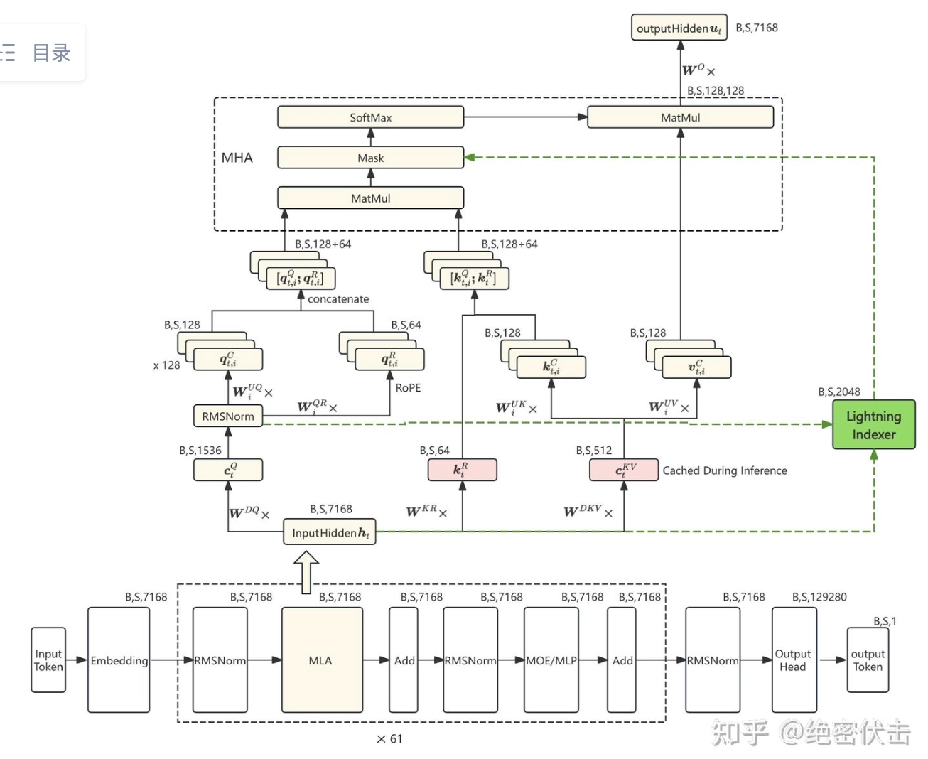
Lightning Indexer 核心逻辑是：将 Q 与 K 进行点积（Matmul），然后对所有 Head 的相关性求和，从而得到每个 Query 与历史 Token 的总体相关性得分。

下面是 Lightning Indexer 的代码实现：

class Indexer(torch.nn.Module):
    def __init__(self, args: ModelArgs):
        super().__init__()
        self.dim: int = args.dim
        self.n_heads: int = args.index_n_heads
        self.n_local_heads = args.index_n_heads // world_size
        self.head_dim: int = args.index_head_dim
        self.rope_head_dim: int = args.qk_rope_head_dim
        self.index_topk: int = args.index_topk
        self.q_lora_rank: int = args.q_lora_rank
        self.wq_b = Linear(self.q_lora_rank, self.n_heads * self.head_dim)
        self.wk = Linear(self.dim, self.head_dim)
        self.k_norm = LayerNorm(self.head_dim)
        self.weights_proj = Linear(self.dim, self.n_heads, dtype=torch.get_default_dtype())
        self.softmax_scale = self.head_dim ** -0.5
        self.scale_fmt = args.scale_fmt
 
        self.register_buffer("k_cache", torch.zeros(args.max_batch_size, args.max_seq_len, self.head_dim, dtype=torch.float8_e4m3fn), persistent=False)
        self.register_buffer("k_scale_cache", torch.zeros(args.max_batch_size, args.max_seq_len, self.head_dim // block_size, dtype=torch.float32), persistent=False)
 
    def forward(self, x: torch.Tensor, qr: torch.Tensor, start_pos: int, freqs_cis: torch.Tensor, mask: Optional[torch.Tensor]):
        bsz, seqlen, _ = x.size()
        end_pos = start_pos + seqlen
        q = self.wq_b(qr)
        q = rearrange(q, 'b s (h d) -> b s h d', d=self.head_dim)
        q_pe, q_nope = torch.split(q, [self.rope_head_dim, self.head_dim - self.rope_head_dim], dim=-1)
        q_pe = apply_rotary_emb(q_pe, freqs_cis)
        q = torch.cat([q_pe, q_nope], dim=-1)
        k = self.wk(x)
        k = self.k_norm(k)
        k_pe, k_nope = torch.split(k, [self.rope_head_dim, self.head_dim - self.rope_head_dim], dim=-1)
        k_pe = apply_rotary_emb(k_pe.unsqueeze(2), freqs_cis).squeeze(2)
        k = torch.cat([k_pe, k_nope], dim=-1)
        q = rotate_activation(q)
        k = rotate_activation(k)
        q_fp8, q_scale = act_quant(q, block_size, self.scale_fmt)
        k_fp8, k_scale = act_quant(k, block_size, self.scale_fmt)
        self.k_cache[:bsz, start_pos:end_pos] = k_fp8
        self.k_scale_cache[:bsz, start_pos:end_pos] = k_scale
        weights = self.weights_proj(x) * self.n_heads ** -0.5
        weights = weights.unsqueeze(-1) * q_scale * self.softmax_scale
        index_score = fp8_index(q_fp8.contiguous(), weights, self.k_cache[:bsz, :end_pos].contiguous(), self.k_scale_cache[:bsz, :end_pos].contiguous())
        if mask is not None:
            index_score += mask
        topk_indices = index_score.topk(min(self.index_topk, end_pos), dim=-1)[1]
        topk_indices_ = topk_indices.clone()
        dist.broadcast(topk_indices_, src=0)
        assert torch.all(topk_indices == topk_indices_), f"{topk_indices=} {topk_indices_=}"
        return topk_indices

DSA计算流 & 性能分析

https://zhuanlan.zhihu.com/p/1963371483985319543

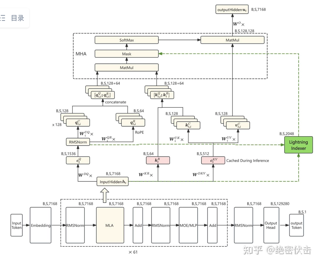
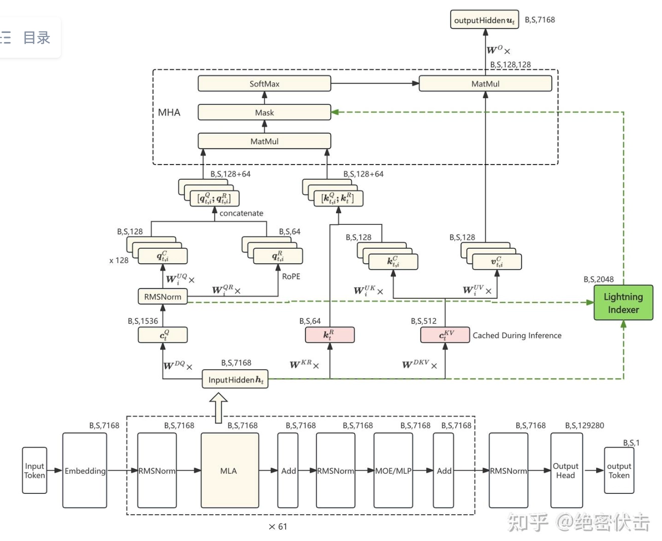
在DeepSeek-V3.2-Exp的技术报告中提到DSA是基于MQA版MLA的改进。对于模式的选择问题，prefill在Top-K内用MHA模式、超过Top-K后用MQA模式，decode用MQA模式。DSA官方示例中prefill采用的MHA模式。考虑到算力特点的介绍，文中prefill用MHA版本、decode用MQA版本。
https://huggingface.co/deepseek-ai/DeepSeek-V3.2-Exp/blob/main/inference/model.py

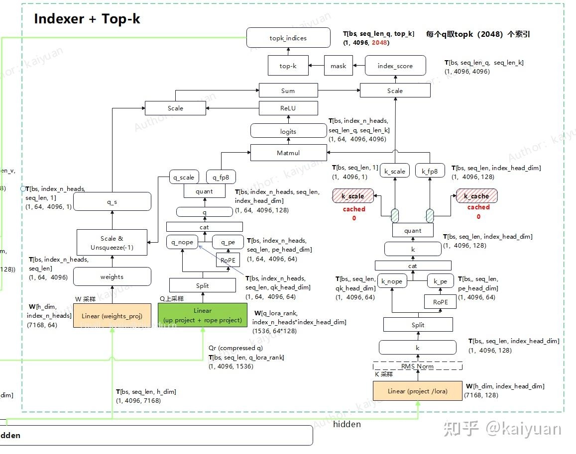
Prefill阶段，以sequence_len=4096为例

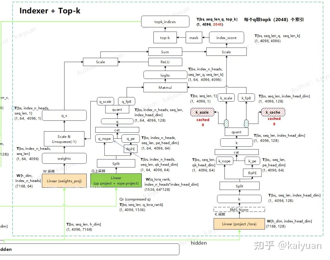
Indexer从左到右主要的三条计算通道分别是w、q、k;
q和k需要计算RoPE，采用采样后拆分单独计算pe后再cat构成整体的q和k;
q、k需要量化处理到FP8，量化值用于计算相关性logits值，由FP8 -> FP32；
k需要做缓存处理，保存量化值和量化比例(scale)；
q的量化scale会先与w进行乘法运算得到q_s, q_s与ReLU的结果相乘；
k的量化scale与Sum相乘；
每个token会有一个topk值，topk默认取2048。当小于该值时，序列全部保留，Indexer模块的计算可以直接绕过。

decode阶段sequence_len=1

Prefill阶段Q的序列长度>1。当序列长度较长时，KV所有tokens都机会被选中，所以Attention计算时，所有的tokens的KV cache都有概率被访问。

KV cache稀疏的实现：

方式1：选择数据加载。若Prefill采用MHA模式，对于每个q token进行QK运算时，需要分头计算。在运算时需要拆解成Q=[1, head_dim]，K=[top-k, head_dim]的AxB矩阵运算，每个头的运算依然独立。如果采用MQA模式，K的head=1，拆解成Q=[heads, 1, head_dim]，K=[top-k, head_dim]的矩阵运算。

注意:两种模式下Attention算子的效率存在差异，若是NV的GPU需要考虑GEMM算子tile的矩阵维度MKN对计算核（Tensor core）的影响，长序列下可能GQA更优。

方式2：通过Mask修改scores，这种方式比较容易实现，但不会节约计算量，不做展开 (也是huggingface上的实现，并不代表真实实现)。

Decode阶段：MLA部分的变化主要是，在KV cache拼接后选择topk个序列进入MQA运算，由于seq_len=1，其它参数不变，所以Decode状态下，当序列长度超过topk设定长度时，MLA部分的计算量不会再增加！

推理

推理主要分为两个阶段，分别是prefill与decode，在prefill阶段，需要计算所有token之间的attention，随后输出第一个token，decode阶段则是自回归的不断输出token，我们分开看这两个阶段：

Prefill

prefill阶段，一般采用MHA的方式；

mla forward

# MLA的forward运算，片段截取-----------------------------:
   def forward(self, x: torch.Tensor, start_pos: int, freqs_cis: torch.Tensor, mask: Optional[torch.Tensor]):
        bsz, seqlen, _ = x.size()
        end_pos = start_pos + seqlen
        qr = self.q_norm(self.wq_a(x))
        q = self.wq_b(qr)
        q = q.view(bsz, seqlen, self.n_local_heads, self.qk_head_dim)
        q_nope, q_pe = torch.split(q, [self.qk_nope_head_dim, self.qk_rope_head_dim], dim=-1)
        q_pe = apply_rotary_emb(q_pe, freqs_cis)
        kv = self.wkv_a(x)
        kv, k_pe = torch.split(kv, [self.kv_lora_rank, self.qk_rope_head_dim], dim=-1)
        kv = self.kv_norm(kv)
        k_pe = apply_rotary_emb(k_pe.unsqueeze(2), freqs_cis)
        self.kv_cache[:bsz, start_pos:end_pos] = kv
        self.pe_cache[:bsz, start_pos:end_pos] = k_pe.squeeze(2)
        if mask is not None:    # MHA prefill
            q = torch.cat([q_nope, q_pe], dim=-1)
            kv = self.wkv_b(kv)
            kv = kv.view(bsz, seqlen, self.n_local_heads, self.qk_nope_head_dim + self.v_head_dim)
            k_nope, v = torch.split(kv, [self.qk_nope_head_dim, self.v_head_dim], dim=-1)
            k = torch.cat([k_nope, k_pe.expand(-1, -1, self.n_local_heads, -1)], dim=-1)
            scores = torch.einsum("bshd,bthd->bsht", q.float(), k.float()) * self.softmax_scale
 
            # indexer 计算获取top k
            topk_indices = self.indexer(x, qr, start_pos, freqs_cis, mask)
            # 此处mask的计算方式是采用直接叠加：
            index_mask = torch.full((bsz, seqlen, seqlen), float("-inf"), device=x.device).scatter_(-1, topk_indices, 0)
            index_mask += mask
            scores += index_mask.unsqueeze(2)
 
            scores = scores.softmax(dim=-1, dtype=torch.float32)
            x = torch.einsum("bsht,bthd->bshd", scores.type_as(x), v)
#  ... 片段截取----------------------------------------

为了降低计算量、显存占用，需要采用定制的算子。在NSA中就提到了优化方案，稀疏attention的kernel计算过程如下图所示，其关键点

Decode

Decode阶段，一般采用MQA的方式，核心出发点是decode时访存密集型，每次只生成一个token，因此核心想法是减少IO操作，因此采用MQA；

训练

由于Lightning Indexer中存在参数如 $w_{t, j}^{I}$ 需要进行训练，以保证后面选取的Top-K的高效性，因而Deepseek训练时采用两阶段训练法

Dense warmup stage：该阶段，仍然采用dense attention的方式，与所有历史token计算attention关系，但训练时，冻结所有的非lightning Indexer外的所有参数，仅训练Lightning Indexer对应参数，；

具体的：对于第 t 个query token，首先通过对主注意力的所有头的attention score进行求和。然后在序列维度上进行 L1 归一化，以产生一个目标分布：

$p_{t,:} = \text{L1-normalized}\left(\sum_{h=1}^{H} \text{AttentionScore}^{(h)}_{t,:}\right)\tag3$

Indexer 产生自身的评分 $I_{t, :}$ ，对其进行 softmax，得到预测分布：

$\hat{p}_{t,:} = \text{Softmax}(I_{t,:})\tag4$

使用 KL 散度 衡量两者之间的差异，作为 Indexer 的训练目标：

$\mathcal{L}^I = \sum_t \text{KL}(p_{t,:} || \hat{p}_{t,:})\tag5$

在此Warm-up Stage，学习率设为 10⁻³ 。仅训练indexer 1000 步，每步包含 16 个 128K 长度的序列，总计处理 2.1 B tokens。
Sparse Training Stage（引入 Sparse Attention）：在此阶段引入细粒度 token 选择机制，并优化所有模型参数，以使模型适应 DSA 的稀疏模式。在此阶段，仍然保持将indexer输出与主注意力分布对齐，但只考虑被选中的token集 $S_{t} = {s ∣ I_{t, s} \in Top-k (I_{t, :})}$

$\mathcal{L}^I = \sum_t \text{KL}(p_{t,S_t} ||\hat{p}_{t,S_t})\tag6$

需要注意的是，将 indexer 的输入从计算图中分离出来，以便进行独立优化。Indexer的训练信号仅来自 $L^{I}$ ，而主模型的优化仅依据语言建模损失。

Sparse Training Stage，学习率设为 7.3 × 10⁻⁶ ，并为每个query token选择2048个 key-value token。同时训练主模型和indexer 15000 步，每步包含 480个128K长度的序列，总计处理 943.7 B tokens。
**Post-Training：**DeepSeek-V3.2-Exp 的后训练阶段在流程、算法和数据上基本延续了 V3.1-Terminus，但在全程中采用了稀疏注意力机制。其核心方法包括：
- 专家蒸馏（Expert Distillation）：针对数学、编程、推理、Agent 等多个专业领域，先分别微调出多个专家模型，然后利用这些专家生成高质量的领域数据，用于蒸馏出一个综合能力更强的统一模型。
- 混合强化学习训练（Mixed RL Training）：采用 GRPO（Group Relative Policy Optimization）算法，将推理、Agent 能力和人类偏好对齐等多个目标统一纳入一个强化学习阶段，有效平衡各领域表现，同时避免多阶段训练常见的灾难性遗忘问题。

Quartz 5

Explorer

DSA (Deepseek Sparse Attention)